Next: Homography Up: Miscellaneous notes Previous: Voronoi tesselation on a Contents
 . As the orthogonal set of sinc functions
 sinc
sinc
 , an analog signal can be (uniquely) produced from a digital signal of length
![$\displaystyle \{ x[n]\}_{n=0}^{N-1}
$](img110.svg)
![$\displaystyle S(t) =\sum_{n = 0}^{N-1} x[n]$](img111.svg) sinc
sinc
 is the sampling rate of the digital signal.
The following GNU Octave function produces the analog signal from a given digital signal
%%Function returns the values at times T of the analog signal of the corresponding digital signal sampled at speed Fs.
function xb = digitaltoanalog(T, digitalsignal, Fs)
  xb = [];
  for t = T
    xb =  [xb sum(digitalsignal.*sinc(Fs*t - (0 : length(digitalsignal) - 1)))];
  end
end
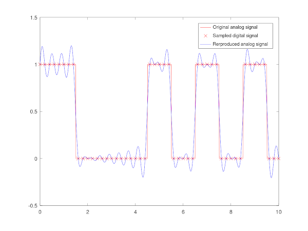
The following code simulates a rectangle pulse train signal given as input, samples the input to a digital signal  , and modulates the sampled digital signal back to an analog signal
  . As the Nyquist rate
restricts the bandwidth of the signal to , information is lost in the sampling stage, because the original rectangle train has an infinite bandwidth.
. As the Nyquist rate
restricts the bandwidth of the signal to , information is lost in the sampling stage, because the original rectangle train has an infinite bandwidth.
pkg load signal;
close all;
clear all;

input  = @(t) pulstran(t,[0,1,5,7,9],"rectpuls") %%The original analog signal at time t.

Fs = 5; %Sampling rate.
t = 10 %Time length of the signal.
Ts = 0 : 1/Fs : t; %Sampling time instances.
x =  input(Ts); %Sampled values, i.e. the digital signal.

Ta = linspace(0, t, 1000); %Analog signal time instances for the plot.
S = digitaltoanalog(Ta, x, Fs); %Modulated analog signal.

%Plot.
plot(Ta, input(Ta), 'color', 'r');
hold on;
plot(Ts, x, 'x', 'color', 'r')
plot(Ta, S, 'color', 'b');
legend( 'Original analog signal','Sampled digital signal', 'Rerproduced analog signal')
References: