Next: Asymptotic decay rate of Up: Miscellaneous notes Previous: May – Digital to Contents
Homography
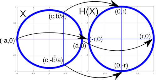
can be used to “change the perspective” of an image (set of vectors). I have used homography for the satellite footprint in the computer simulations. For elevation angles smaller than
 , you can conveniently map transmitters inside the elliptical footprint to a circle for which the radially symmetric antenna pattern function can be used. The following homography matrix
  transforms an ellipse
of parameters
transforms an ellipse
of parameters  and
and  to a circle of radius
  so that the right-hand side focus point maps to the origin.

Here is a GNU Octave code:
%%Changes ellipses with parameters a > b  perspective to a sphere of radius r centered in origo. Vectors to be transformed are given in 2x1000 matrix refc.

function points = homography(refc, a,b,r)
  c = sqrt(a^2 - b^2);
  %%Construct the homography matrix.
  X1 = [[-a -0 -1 0 0 0 a*r 0*r r]; [0 0 0 -a -0 -1 a*0 0*0 0]];
  X2 = [[-c -b^2/a -1 0 0 0 c*0 b^2/a*0 0]; [0 0 0 -c -b^2/a -1 c*r b^2/a*r r]];
  X3 = [[a 0 -1 0 0 0 -a*-r 0*-r -r]; [0 0 0 a -0 -1 -a*0 0*0 0]];
  X4 = [[-c b^2/a -1 0 0 0 c*0 -b^2/a*0 0]; [0 0 0 -c b^2/a -1 c*-r b^2/a*r -r]];
  P = [X1; X2; X3; X4];
  [U,S,V] = svd(P); %Singular value composition.
  h = V(:,9);
  H = reshape(h, 3, 3)';
  points = [];
  for point = refc
    homopoint = [point; 1]; %Point presented in homogeneous coordinates.
    homopoint = H*homopoint;
    homopoint = [homopoint(1)/homopoint(3); homopoint(2)/homopoint(3)];
    points = [points homopoint];
  end
  figure(1)
  plot(points(1,:), points(2,:), 'b','linewidth',10);
end
In the following, we are rotating a “pyramid”. It can be seen how the homography mapping can be interpreted as a change of perspective.
References: