Next: June Why does MIMO Up: Blog posts 2021 Previous: March Signal propagation in Contents
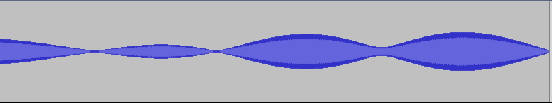
When a signal propagates through multiple paths, each signal component in each path will be in a different phase and of varying strength when received. Should there be no line-of-sight component present, the additive signal will fade according to the Rayleigh fading.
For example, a simple sine wave
wave (links to soundcloud.com—VOLUME ALERT)
can after some multi-path propagation sound like
this:
Assuming that the receiver is moving, the variation of Doppler shifts in different signal paths will cause the signal strength to vary randomly in time.
If we add some Gaussian white noise, we notice that the original signal is somehow recognizable from the
noised signal (listen carefully, and you will hear the sine signal in the background).
but the
will sometimes get buried under the noise—these events are referred to as deep fades.
 |
Here is a GNU Octave or Matlab code for the used Rayleigh simulator, which outputs the signal as audio:
%Rayleigh simulator. Jakes model. In Octave remember to load the statistics package.

close all
clear all

tic

N = 20; %Number multipaths.
T = linspace(0,10000,100000); %Time.
v = 0.001; %Speed of the receiver.
randan = pi*rand(1,N); %Random angles w.r.t. receiver.
rI = 1000*rand(1,N); %Random distances of the sources.

%Geometrical stuff. Check for the Jakes model in the reference.
An = @(t) (atan(sin(randan).*rI./(cos(randan).*rI-v*t))).*(cos(randan).*rI>v*t)+...
(pi-atan(sin(randan).*rI./(v*t-cos(randan).*rI))).*(cos(randan).*rI<=v*t);
phis = 2*pi.*(rand(1,N));
wc =pi/2; %Frequency of the signal.
Beta = 2*pi/(1/(wc/(2*pi)));
theta = @(t) cos(An(t)).*Beta*v.*t+phis;

powers = rand(1,N); %Random powers of the signals in the multipaths.
powers = powers./sum(powers); %Normalize the powers.
Ez = @(t) sum(powers.*cos(wc*t+theta(t)));
EZ = []; %Faded signal.
REF = []; %Original signal.
NOISE = []; %Additional Gaussian noise.
for t =T
EZ = [EZ Ez(t)];
REF = [REF cos(wc*t)];
NOISE = [NOISE 0.9*stdnormal_rnd(1)];
end

%Write the audio files at sampling rate 8000.
audiowrite('EZ.wav',EZ,8000)
audiowrite('EZNOISE.wav',1/2*(EZ+NOISE),8000)
audiowrite('REFNOISE.wav', 1/2*(REF+NOISE), 8000)


toc
plot(T,EZ)
And the same in Python:
  import numpy as np
  import math
  import matplotlib.pyplot as plt
  import sounddevice as sd
  import time

  #Jakes Rayleigh simulator. Please check for the reference in this site for further details.

  N = 20 #Number of multipaths.
  T = np.linspace(0, 10000, 100000) #Time vector.
  v = 0.001 #Speed of the receiver.


  randan = np.random.rand(1, N) * math.pi #Random angles w.r.t. receiver.
  rI = np.random.rand(1, N) * 1000 #Random distances of the sources.
  phis = np.random.rand(1, N) * 2 * math.pi

  def An(t):
  return (np.arctan(np.sin(randan) * rI / (np.cos(randan) * rI - v * t))) * (
  np.cos(randan) * rI > v * t
  ) + (np.pi - np.arctan(np.sin(randan) * rI / (v * t - np.cos(randan) * rI))) * (
  np.cos(randan) * rI <= v * t
  )

  wc = np.pi/2 #Frequency of the signal.
  Beta = 2 * math.pi / (1 / (wc / (2 * math.pi)))

def theta(t):
    return np.cos(An(t)) * Beta * v * t +phis

powers = np.random.rand(1,N)*2 #Random powers of the signals in the multipaths.
powers = powers/np.sum(powers) #Normalize powers..

def Ez(t):
    return np.sum(powers * np.cos(wc * t + theta(t)))

EZ = np.vectorize(Ez)(T)
REF = np.vectorize(lambda time : 2*np.cos(wc * time))(T)

#Play and plot.
fs = 8000
sd.play(EZ,fs,blocking = True)
#sd.play(REF,fs,blocking = True)
plt.plot(T, EZ)
plt.show()
References: