Next: Blog posts 2022 Up: Blog posts 2023 Previous: Blog posts 2023 Contents
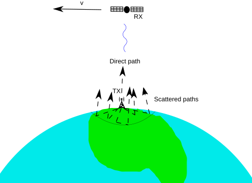
Let us study a faded signal in an omnidirectional satellite receiver sent by an earth transmitter. We consider that the transmitter (TX) is sending a constant QAM symbol, i.e., the TX baseband signal is given by
 |
( ) ) |
![$\theta \in [0,1]$](img45.svg) and
and
 . The passband signal
experiences fading
due to terrestrial obstacles. We use a model where
. The passband signal
experiences fading
due to terrestrial obstacles. We use a model where  scatterer objects are Poisson distributed
inside a circular area with a diameter of
scatterer objects are Poisson distributed
inside a circular area with a diameter of  m. The phases of the scattered signals are independently uniformly random. Initially, the satellite, which is moving at its orbital speed, is in the zenith
w.r.t. the earth transmitter. The receiver's (RX) baseband signal is a linear combination of the down-conversions
of the scattered, Doppler shifted
and attenuated
passband signal components, and it is given by
m. The phases of the scattered signals are independently uniformly random. Initially, the satellite, which is moving at its orbital speed, is in the zenith
w.r.t. the earth transmitter. The receiver's (RX) baseband signal is a linear combination of the down-conversions
of the scattered, Doppler shifted
and attenuated
passband signal components, and it is given by
 |
(2) |
 is the path-loss function at distance
  from the scatterer
  ,
,  is the direct-path distance to the transmitter,
  is the parameter that determines the energy ratio of the direct-path (LOS) component and the scattered paths, and
 is the propagation delays restricted by the speed of light
  , which is dependent on time
  as the satellite moves, and
  is the carrier frequency.
Given this model, we are interested in the time scale during which
 varies, i.e., the coherence time. The coherence time depends on the Doppler shift, and the satellite's orbital speed is given by
 |
(3) |
 m
m s
s , and the denominator is the sum of the satellite's altitude and the earth's radius, respectively. This is fast: around
  km/s at
  km. However, Doppler shift is only caused by the velocity component that is directed towards the transmitter. The Doppler shift is zero when the satellite is in the zenith and grows at lower elevation angles. In our model, the scatterers were distributed in an area of diameter m below the satellite, and the maximum Doppler shift initially is
  Hz for
 ; hence, the Doppler spread is
  Hz. A small estimate for the coherence time is given by
 s s |
(4) |
 meters during this period.
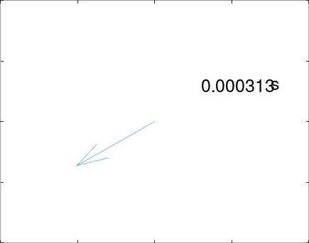
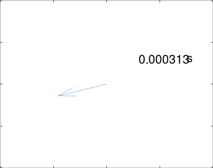
The following figures illustrate the RX baseband signal changing in time while the satellite moves. As expected, the variance in the signal strength is larger in the Rayleigh faded case.
Here is the Octave code:
function signals = satellite_baseband_simulation()
  pkg load statistics
  close all;
  clear all;
  clear imread;
  clear imwrite;

  h = 600*1000; #Altitude of satellites.
  K = 0; #Rician parameter.
  t = 0; #Initial time.
  [refs bbsignals] = scatteredsignals(K);  #Random baseband signals ”bbsignals' and the scatterer-obstacle's locations in 'refs'.
  signal = RXbaseband(refs, bbsignals);
  N = 200;
  history =[];
  filename = 'basebandgif.gif';
  if(exist(filename))
    delete(filename);
  end


  for iii = 1 : N
    ##Observe the progress.
    if(mod(iii,10) == 0)
      iii
    end
    refs = rotateearth(refs); #Rotate Earth.
    signal = RXbaseband(refs, bbsignals); #New received baseband signal
    history = [history [real(signal); imag(signal)]]; #History of the signals.
    ##Write GIF.
    quiver(0,0,real(signal), imag(signal));
    hold on;
    plot(history(1,:), history(2,:))
    axis([[-0.1, 0.1], [-0.1, 0.1]]);
    t = t + 1/(4*8*100); #Time hop. t = 1/(8*300) is the initial coherence time of the example.
     text(0.03, 0.03, mat2str(t, 3), 'fontsize',25);
    text(0.075, 0.03, 's', 'fontsize',25);
    frame = getframe();
    imwrite(frame.cdata, filename,'gif','writemode','append','DelayTime',0.05, 'Compression','lzw')
    hold off;
  end
end


##Returns a table of 101 (1 LOS signal and 100 signals from the scattered paths) randomly phased complex baseband signal symbols each corresponding to one of a obstacle location given in 'refs'. 'K' is the Rician parameter.
function [refs, signals] = scatteredsignals(K)
  ##First, generate the Poisson distributed random obstacle locations.
  refs = [0; 0]; #LOS component.
  yMin = 1-0.0000000001; yMax = 1;
  xMin = -pi; xMax = pi;
  xDelta = xMax - xMin; yDelta = yMax - yMin; #Rectangle dimensions
  numbPoints =100;    #Number of points.
  x = xDelta*(rand(numbPoints,1)) + xMin;    #Pick points from uniform distribution
  y = yDelta*(rand(numbPoints,1)) + yMin;
  refs = [refs [pi/2-asin(y)' ; x'] ]; #Map referencepoints to spherical coordinates
  A = 30000; #Amplitude.
  signals = [A*sqrt(K/(K+1)).*exp(-rand(1,1).*i*2*pi)];
  signals = [signals A/(sqrt(100)*sqrt(1+K)).*exp(-rand(1,length(refs(1,:))-1).*i*2*pi)];
end


##Derives the received baseband signal.
function bb = RXbaseband(refs, signals)
  R = 6378*1000; #Radius of Earth in m.
  h = 600*1000; #Altitude of the satellite.
  d = @(gamma) sqrt((cos(gamma).*(R+h)-R).^2+(sin(gamma).*(R+h)).^2); ##Distance to the satellites in m.
  c = 299792458; ##Speed of light.
  if(!isempty(refs))
    a = 1./d(refs(1,:));
    tau  = d(refs(1,:))/c;
  else
    a = 0;
    tau = 0;
  end
  fc = 12*10^9; ##Modulation frequency.
  ab = a.*exp(-i*2*pi*tau.*fc); ##Received individual signals.
  bb = sum(ab.*signals); ##Aggregate received signal.
end

##Rotates the positions in 'refs' as the satellite "moves". In this model, the satellite stays still at (0,0) but the Earth moves.
function refs = rotateearth(refs)
  t = 1/(4*8*100); #Time hop in seconds.
  h= 600*1000; #Altitude of the satellite.
  R = 6378*1000; #Radius of Earth.
  GM = 3.986*10^14; #Gravitational constant.
  orbitalspeed = sqrt(GM/(h + R)); #Satellite speed in m/s.
  angularspeed = orbitalspeed/(h + R); #Angular speed of the satellite.
  rotation = angularspeed*t; #Rotation of Earth.
  eucpos  = pol2euc(refs); #Transform the polar coordinates to euclidean coordinates.
  newpos = [[1 0 0]; [0 cos(rotation) -sin(rotation)]; [0 sin(rotation) cos(rotation)]]*eucpos; #Rotation about x-axis.
  refs = euc2pol(newpos); #Back to the polaroordinates.
end


function p  = euc2pol(e)
  R = 6378*1000; #Radius of Earth.
  p = [acos(e(3,:)./R); (e(2,:) >= 0).*atan2(e(2,:),e(1,:)) + ...
			(e(2,:) < 0).*(atan2(e(2,:),e(1,:)) + 2*pi)]; #Polar coordinates from the given Euclidean coordinates in 'e'..
end

function e = pol2euc(p)
  R= 6378*1000; #Radius of Earth.
  e = [R*cos(p(2,:)).*sin(p(1,:));...
       R*sin(p(2,:)).*sin(p(1,:));...
       R*cos(p(1,:))]; #Euclidean coordinates from the given polar coordinates in 'p'.
end
References: